TUBE UNDERDEVELOPEDYouTube ↗
EPISODE 02 · AN ANIMATED JOURNEY

Seventeen equations.
A new way to see.

From the length of a diagonal to the price of a promise. Discover the questions, ideas and people behind the mathematics that shapes our world.

17:47English narration
English & Chinese subtitles

The complete film · 17 minutes of mathematical discovery

Watch on YouTube ↗

THE JOURNEY

Follow a question.

Choose a chapter to jump to that moment in the film.

THE IDEAS, UP CLOSE

A world in seventeen chapters.

Each formula begins with something we want to understand.

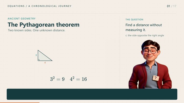
Animated illustration of Pythagorean theorem▶ 00:26
01 / 17 Ancient geometry

Pythagorean theorem

Two known sides. One unknown distance. A right triangle turns a practical question into a lasting mathematical relationship.

a2+b2=c2a^2+b^2=c^2
A closer look

The right angle lies between a and b. Babylonian knowledge predates the traditional association with Pythagoras.
Watch this chapter
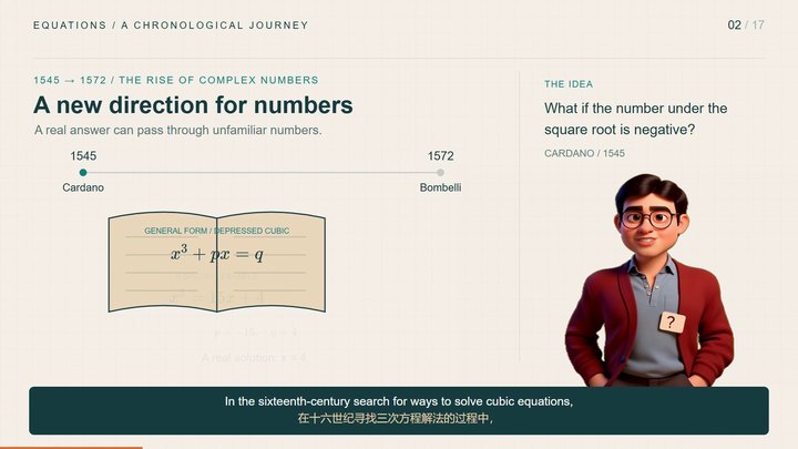
Animated illustration of Complex numbers▶ 01:12
02 / 17 1545 → 1572

Complex numbers

A real answer can take a surprising route through complex numbers. Cardano and Bombelli helped make that route usable.

x3+px=qi2=−1x^3+px=q\qquad i^2=-1
A closer look

The example x³ = 15x + 4 has x = 4. The paired complex cube roots 2+i and 2−i add to 4.

Watch this chapter
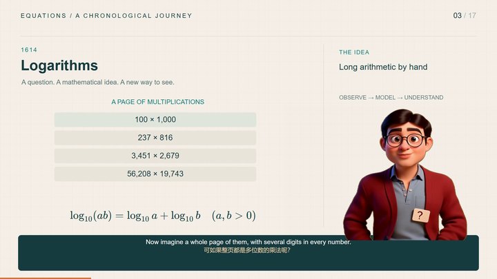
Animated illustration of Logarithms▶ 02:08
03 / 17 1614

Logarithms

What if multiplication could become addition? Logarithms made long calculations more manageable.

log⁡b(xy)=log⁡bx+log⁡by\log_b(xy)=\log_b x+\log_b y
A closer look

For x,y > 0 and a common base b > 0, b ≠ 1.

Watch this chapter
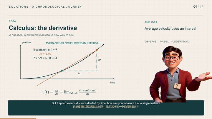
Animated illustration of Calculus▶ 03:02
04 / 17 The seventeenth century

Calculus

A speedometer asks about change right now. The derivative connects an interval of change to an instantaneous rate.

f′(t)=lim⁡h→0f(t+h)−f(t)hf\prime(t)=\lim_{h\to0}\frac{f(t+h)-f(t)}{h}
A closer look

Newton and Leibniz independently developed calculus. The visual example uses position f(t)=t².

Watch this chapter
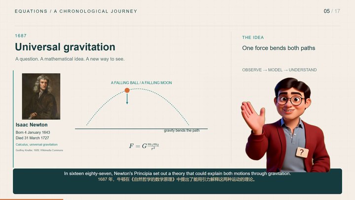
Animated illustration of Universal gravitation▶ 04:01
05 / 17 1687

Universal gravitation

A thrown ball and an orbiting Moon share a question: what bends their paths? Newton connected them with one law.

F=Gm1m2r2F=G\frac{m_1m_2}{r^2}
A closer look

The inverse-square expression applies to point masses; the orbit illustration is schematic.

Watch this chapter
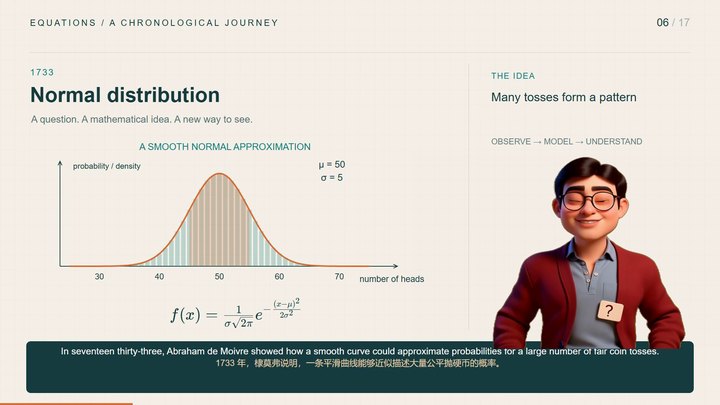
Animated illustration of Normal distribution▶ 04:57
06 / 17 1733 and later developments

Normal distribution

Many small uncertainties can form a familiar bell-shaped pattern. Probability makes that pattern measurable.

f(x)=1σ2πe−(x−μ)22σ2f(x)=\frac{1}{\sigma\sqrt{2\pi}}e^{-\frac{(x-\mu)^2}{2\sigma^2}}
A closer look

The animation compares 100 fair coin tosses with a normal approximation: mean 50, standard deviation 5.

Watch this chapter
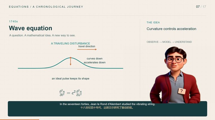
Animated illustration of Wave equation▶ 05:51
07 / 17 1746

Wave equation

Pluck a string and a disturbance travels. Local curvature and acceleration connect to describe a moving wave.

∂2u∂t2=c2∂2u∂x2\frac{\partial^2u}{\partial t^2}=c^2\frac{\partial^2u}{\partial x^2}
A closer look

An ideal one-dimensional linear wave model; fixed ends introduce standing waves.

Watch this chapter
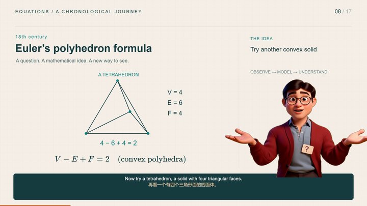
Animated illustration of Euler polyhedron formula▶ 06:46
08 / 17 The eighteenth century

Euler polyhedron formula

Count corners, edges and faces. Changing a polyhedron can preserve a relationship hidden in those counts.

V−E+F=2V-E+F=2
A closer look

For convex polyhedra. Adding a diagonal across one face increases both E and F by one.

Watch this chapter
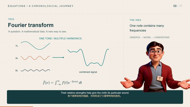
Animated illustration of Fourier transform▶ 07:38
09 / 17 1822

Fourier transform

A single sound can contain many simple waves. Fourier analysis reveals the frequencies inside a signal.

f^(ν)=∫−∞∞f(t)e−2πiνt dt\widehat f(\nu)=\int_{-\infty}^{\infty}f(t)e^{-2\pi i\nu t}\,dt
A closer look

The demonstration combines three harmonics. The displayed transform uses frequency ν and the 2π convention.

Watch this chapter
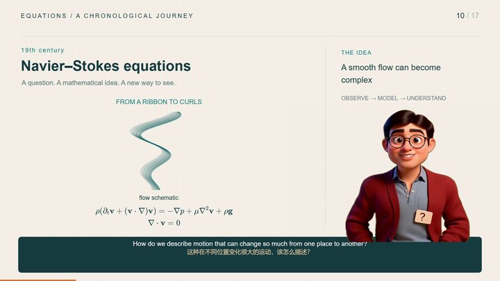
Animated illustration of Navier-Stokes equations▶ 08:35
10 / 17 The nineteenth century

Navier-Stokes equations

Smoke curls, water flows, and neighbouring layers pull on one another. A fluid equation balances the forces.

ρ(∂u∂t+u⋅∇u)=−∇p+μ∇2u+ρg\rho\left(\frac{\partial\mathbf u}{\partial t}+\mathbf u\cdot\nabla\mathbf u\right)=-\nabla p+\mu\nabla^2\mathbf u+\rho\mathbf g
A closer look

Incompressible Newtonian fluid with constant density and viscosity, ∇·u=0. The streamlines are illustrative, not a numerical PDE solution.

Watch this chapter
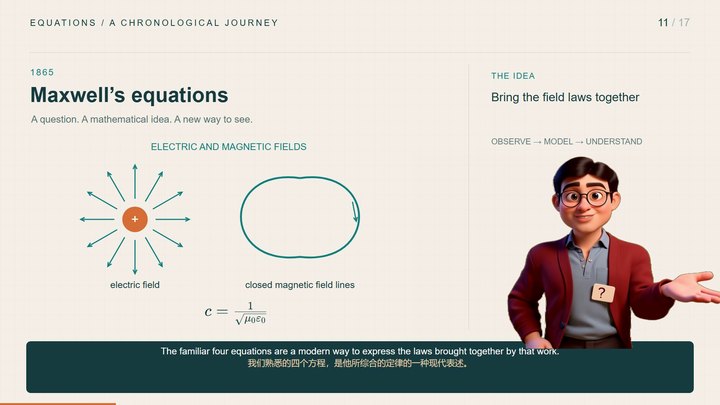
Animated illustration of Maxwell equations▶ 09:41
11 / 17 1865

Maxwell equations

Electricity and magnetism become one picture. Changing fields can sustain waves that travel through empty space.

∇⋅E=ρ/ϵ0∇⋅B=0∇×E=−∂tB∇×B=μ0J+μ0ϵ0∂tE\begin{aligned}\nabla\cdot\mathbf E&=\rho/\epsilon_0&\nabla\cdot\mathbf B&=0\\\nabla\times\mathbf E&=-\partial_t\mathbf B&\nabla\times\mathbf B&=\mu_0\mathbf J+\mu_0\epsilon_0\partial_t\mathbf E\end{aligned}
A closer look

Modern SI notation. In vacuum, c=1/√(μ₀ε₀); the electric and magnetic fields in a plane wave are transverse and in phase.

Watch this chapter
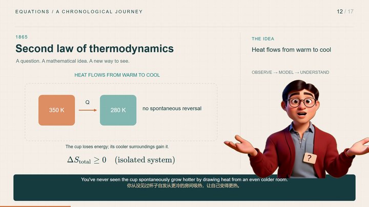
Animated illustration of Second law of thermodynamics▶ 10:43
12 / 17 The nineteenth century

Second law of thermodynamics

Heat spreads from warm to cool. The second law gives that everyday direction a mathematical expression.

ΔSisolated≥0\Delta S_{\mathrm{isolated}}\geq0
A closer look

For an isolated system. The example conserves energy while the total entropy of two bodies increases.

Watch this chapter
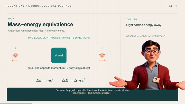
Animated illustration of Mass-energy equivalence▶ 11:35
13 / 17 1905

Mass-energy equivalence

Mass and rest energy are connected. Even a tiny difference in mass can correspond to an enormous amount of energy.

E0=mc2E_0=mc^2
A closer look

Equal opposite light pulses carry energy away without net momentum; the body loses mass.

Watch this chapter
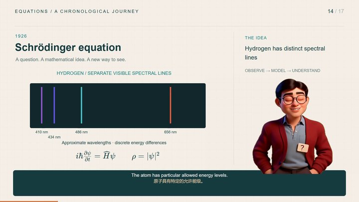
Animated illustration of Schrodinger equation▶ 12:34
14 / 17 1926

Schrodinger equation

Atoms emit distinct colours. Quantum mechanics replaces a classical path with a state that evolves in time.

iℏ∂ψ∂t=H^ψi\hbar\frac{\partial\psi}{\partial t}=\widehat H\psi
A closer look

The free wave packet and hydrogen energy levels are separate examples. Hydrogen n=3→2 emits about 1.89 eV, near 656 nm.

Watch this chapter
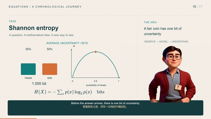
Animated illustration of Shannon entropy▶ 13:36
15 / 17 1948

Shannon entropy

A predictable message tells us less. Shannon quantified uncertainty and opened a new way to think about information.

H(X)=−∑xp(x)log⁡2p(x)H(X)=-\sum_x p(x)\log_2p(x)
A closer look

Base-two logarithms give entropy in bits. A binary source with probabilities .95 and .05 has about .286 bits of entropy.

Watch this chapter
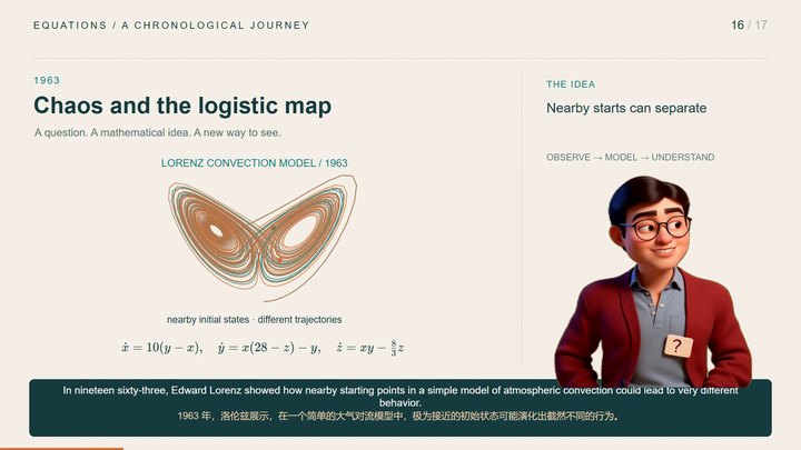
Animated illustration of Chaos and logistic map▶ 14:33
16 / 17 1963 and later examples

Chaos and logistic map

Simple rules can produce complicated behaviour. Nearby starting points may lead to very different futures.

xn+1=R xn(1−xn)x_{n+1}=R\,x_n(1-x_n)
A closer look

Lorenz’s continuous convection system is distinct from the logistic map. The latter illustrates stable, periodic and chaotic behaviour.

Watch this chapter
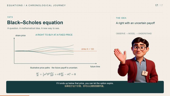
Animated illustration of Black-Scholes equation▶ 15:38
17 / 17 1973

Black-Scholes equation

How do we value a promise with an uncertain payoff? A model links an option’s price to the risks it can hedge.

∂C∂t+12σ2S2∂2C∂S2+rS∂C∂S−rC=0\frac{\partial C}{\partial t}+\frac12\sigma^2S^2\frac{\partial^2 C}{\partial S^2}+rS\frac{\partial C}{\partial S}-rC=0
A closer look

European options under the Black–Scholes assumptions. An illustrative model price is not a forecast or investment recommendation.

Watch this chapter

A SHARED HUMAN STORY

The people behind the equations.

Namesakes, pioneers and contributors. Discovery rarely belongs to one person alone.

Ancient dates are approximate. The image of Pythagoras is a later imagined likeness; Bombelli is represented by a historical book title page. Living contributors are identified as living.

Meet the 23 people in the tribute
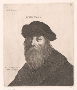
Pythagoras — historical image

Pythagoras

Born c. 570 BCE · Died c. 490 BCE

Traditional namesake; earlier Babylonian knowledge

Rijksmuseum; Jerome David after Claude Vignon · Image source · CC0. Resized for web display.

Later imagined likeness, not a contemporary portrait. Dates are approximate.

Biography ↗
Gerolamo Cardano — historical image

Gerolamo Cardano

Born 24 September 1501 · Died 21 September 1576

Published Ars Magna (1545)

Library of Congress; anonymous historical engraving · Image source · Public domain. Resized for web display.

Complex numbers developed through several contributors.

Biography ↗
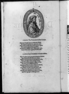
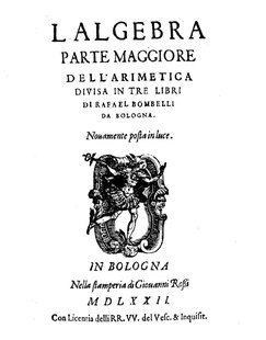
Rafael Bombelli — book title page

Rafael Bombelli

Born January 1526 · Died 1572

Rules for complex arithmetic (1572)

Rafael Bombelli, Algebra (1572); BEIC / Wikimedia Commons · Image source · Public domain. Resized for web display.

BOOK TITLE PAGE, not a portrait. Exact birth/death days are not established here; 20 January 1526 is a baptism date.

Biography ↗
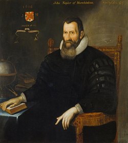
John Napier — historical image

John Napier

Born 1550 · Died 4 April 1617

Published logarithms (1614)

Unknown artist, 1616; Wikimedia Commons · Image source · Public domain. Resized for web display.

Birth month and day are not reliably established.

Biography ↗
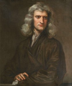
Isaac Newton — historical image

Isaac Newton

Born 4 January 1643 · Died 31 March 1727

Calculus; universal gravitation

Godfrey Kneller, 1689; Wikimedia Commons · Image source · Public domain. Resized for web display.

Gregorian dates. Old Style dates: 25 December 1642 and 20 March 1727.

Biography ↗
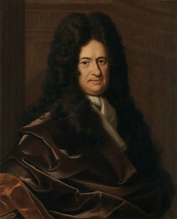
Gottfried Wilhelm Leibniz — historical image

Gottfried Wilhelm Leibniz

Born 1 July 1646 · Died 14 November 1716

Independent co-developer of calculus

Christoph Bernhard Francke, c. 1695; Wikimedia Commons · Image source · Public domain. Resized for web display.

Birth date is Gregorian.

Biography ↗
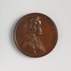
Abraham de Moivre — historical image

Abraham de Moivre

Born 26 May 1667 · Died 27 November 1754

Early normal approximation (1733)

Jacques-Antoine Dassier; The Metropolitan Museum of Art / CC0 · Image source · CC0. Resized for web display.

Primary figure named in the narration.

Biography ↗
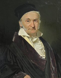
Carl Friedrich Gauss — historical image

Carl Friedrich Gauss

Born 30 April 1777 · Died 23 February 1855

Normal distribution: later development

Christian Albrecht Jensen, 1840; Wikimedia Commons · Image source · Public domain. Resized for web display.

Optional supporting figure; do not replace de Moivre in the 1733 narration.

Biography ↗
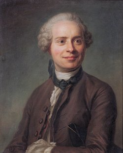
Jean le Rond d’Alembert — historical image

Jean le Rond d’Alembert

Born 17 November 1717 · Died 29 October 1783

Vibrating string and wave equation

French school, after Maurice Quentin de La Tour; Wikimedia Commons · Image source · Public domain. Resized for web display.

The ideal wave equation developed through several contributors.

Biography ↗
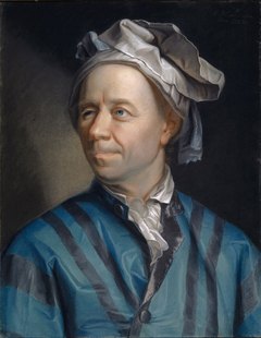
Leonhard Euler — historical image

Leonhard Euler

Born 15 April 1707 · Died 18 September 1783

Polyhedral relation: V - E + F = 2

Jakob Emanuel Handmann; Kunstmuseum Basel / Wikimedia Commons · Image source · Public domain. Resized for web display.

Dates follow the cited biography.

Biography ↗
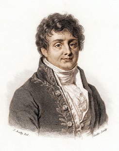
Joseph Fourier — historical image

Joseph Fourier

Born 21 March 1768 · Died 16 May 1830

Heat theory and harmonic analysis

Julien-Leopold Boilly; restored image / Wikimedia Commons · Image source · Public domain. Resized for web display.

The modern Fourier transform developed beyond Fourier’s original work.

Biography ↗
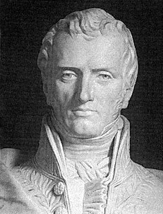
Claude-Louis Navier — historical image

Claude-Louis Navier

Born 10 February 1785 · Died 21 August 1836

Viscous fluid equations

Historical portrait; Wikimedia Commons · Image source · Public domain. Resized for web display.

Low-resolution historical portrait: 231 x 303 pixels.

Biography ↗
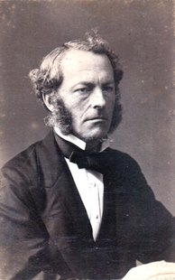
George Gabriel Stokes — historical image

George Gabriel Stokes

Born 13 August 1819 · Died 1 February 1903

Viscous fluid equations

Unidentified photographer; Smithsonian Institution Libraries · Image source · No restrictions. Resized for web display.

Smithsonian declares no known copyright restrictions; this is not a CC0 dedication.

Biography ↗
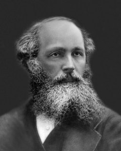
James Clerk Maxwell — historical image

James Clerk Maxwell

Born 13 June 1831 · Died 5 November 1879

Electromagnetic field theory (1865)

Unknown historical photographer; Wikimedia Commons · Image source · Public domain. Resized for web display.

Unified earlier laws; familiar four-equation notation is a later form.

Biography ↗
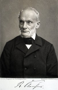
Rudolf Clausius — historical image

Rudolf Clausius

Born 2 January 1822 · Died 24 August 1888

Second law and entropy

Theodor Schafgans; Wikimedia Commons · Image source · Public domain. Resized for web display.

Primary figure in this narration; not an attribution of all thermodynamics to one person.

Biography ↗
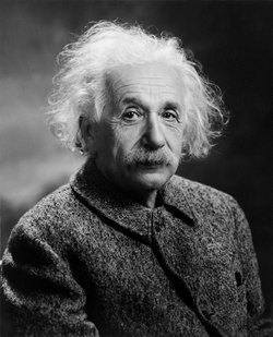
Albert Einstein — historical image

Albert Einstein

Born 14 March 1879 · Died 18 April 1955

Mass-energy equivalence (1905)

Oren Jack Turner, 1947; Wikimedia Commons · Image source · Public domain. Resized for web display.

Image is a later-life portrait, photographed in 1947.

Biography ↗
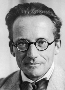
Erwin Schrödinger — historical image

Erwin Schrödinger

Born 12 August 1887 · Died 4 January 1961

Wave mechanics (1926)

Unknown photographer; Narodowe Archiwum Cyfrowe · Image source · Public domain. Resized for web display.

Historical archival photograph.

Biography ↗
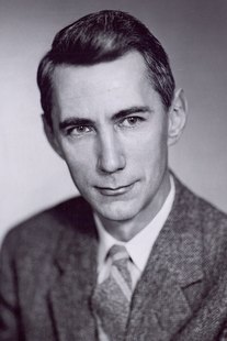
Claude Shannon — historical image

Claude Shannon

Born 30 April 1916 · Died 24 February 2001

Information theory and entropy (1948)

Unknown photographer; Tekniska museet / CC BY 2.0 · Image source · CC BY 2.0. Resized for web display.

Attribution required under CC BY 2.0.

Biography ↗
Edward Norton Lorenz — historical image

Edward Norton Lorenz

Born 23 May 1917 · Died 16 April 2008

Deterministic chaos (1963)

American Geophysical Union, courtesy of AIP Emilio Segre Visual Archives · Image source · Attribution. Resized for web display.

Do not credit Lorenz as inventor of the logistic map. AIP attribution permission permits reuse.

Biography ↗
Robert McCredie May — historical image

Robert McCredie May

Born 8 January 1936 · Died 28 April 2020

Logistic-map chaos: influential 1976 exposition

NBeale / English Wikipedia; CC BY-SA 3.0 · Image source · CC BY-SA 3.0. Resized for web display.

Optional supporting figure for the logistic-map illustration; not a claim that he invented the map.

Biography ↗
Fischer Black — historical image

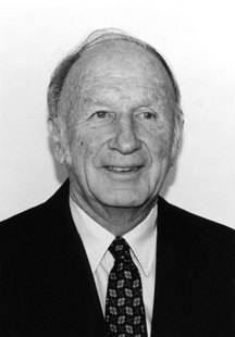
Fischer Black

Born 11 January 1938 · Died 30 August 1995

Option pricing: Black-Scholes (1973)

Dalmatine / English Wikipedia; public-domain dedication · Image source · Public domain. Resized for web display.

Author released the photograph into the public domain.

Biography ↗
Myron Scholes — historical image

Myron Scholes

Born 1 July 1941 · Living

Option pricing: Black-Scholes (1973)

Nobellaureatesphotographer / English Wikipedia; CC BY-SA 3.0 · Image source · CC BY-SA 3.0. Resized for web display.

Living as of the research date. Use a tribute caption, not a death memorial.

Biography ↗
Robert C. Merton — historical image

Robert C. Merton

Born 31 July 1944 · Living

Option pricing: continuous-time extension

Massachusetts Institute of Technology / CC BY-SA 4.0 · Image source · CC BY-SA 4.0. Resized for web display.

Optional supporting figure. Living as of the research date.

Biography ↗

KEEP EXPLORING

Read. Listen. Look closer.

Return to a formula, download the English captions, or explore the original scientific references.

The soundtrack

Original selections from the creator’s Mureka AI-generated music library.

  • Evolving Horizons
  • Electric Dawn
  • Aqueous Reverie
  • The Quiet Beauty of Equations
  • Patterns of Wonder
  • From Numbers to the Cosmos

How was this made?

A behind-the-scenes tutorial is planned: research, narration, mathematical animation, bilingual captions, AI-generated music and the final edit.

Tell us what you’d like to learn ↗